Introduction to Source Extraction
MExtract Module
This tutorial shows you how use the MExtract module to detect and measure the properties of sources in one or more images. The MExtract tool is accessed using the Measure > Extract Sources command for an Image Window. The MExtract module is immensely powerful and has a great number of important and varied applications. In this tutorial it is used simply to examine the FWHM values for many stars in a small region of an astronomical image. A quick overview of the extraction procedure is also described in Running the Source Extraction Pipeline.
Source extraction involves the detection and measurement of all objects brighter than a threshold value. This processing uses a chain of operations called a "pipeline". Each step in the pipeline involves preferences that control its operation. Because Mira allows so many variations for the steps used in the pipeline, a Profile control is used to manage the procedure. The pipeline is operated from the Source Extraction Dialog. After you have choose a profile or set your preferences, you run the pipeline by clicking the [Process] button.
The source extraction pipeline involves a procedure consisting of the steps you want to use. Each of these steps is optional but those you select are applied in a specific order, hence the term "pipeline" to describe a single direction of flow in the processing. The first step in source extraction involves determination of the background level. Knowing the background at each point, each pixel can be tested against the threshold above background; if the pixel exceeds the threshold, it is tagged as a source candidate. All candidate pixels are then collected into objects completely separated from others by a boundary at the specified threshold level. In this way, the sources are like islands poking above sea level. Source properties such as luminance, ellipticity, area, and others are then computed. The final processing step involves filtering this source list to retain only the sources that meet criteria such as being within a certain range of area or ellipticity. The list of sources extracted from the image(s) may then be further analyzed using Mira tools or saved for analysis by other software.
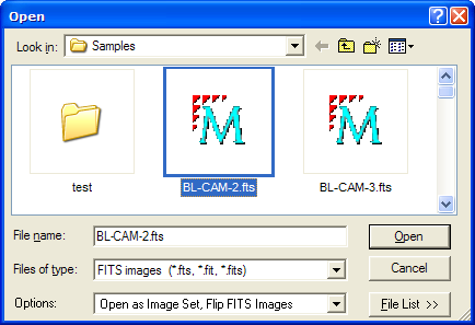
To begin, use the File > Open command to load the Open dialog. As shown below, select the sample image BL-CAM-2.fts and click [Open] to display it in Mira.
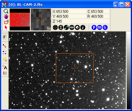
After opening the image, click the Measure > Extract Sources command in the pull-down menu. This opens the Source Extraction Toolbar which operates all the commands of the Source Extraction package. As typical in Mira, the toolbar opens on the left border of the image window with marking mode active:
The toolbar commands are described below. In this tutorial, the only buttons you will use are the first and last ones:
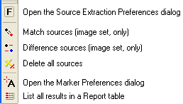
Notice that there is no marking mode on this toolbar. This is different from the way most command toolbars work because source extraction does not involve any interactive marking modes. Rather than clicking on sources using the mouse, source extraction automatically finds the objects for you.
Next, we will load the extraction preferences to be
used in this tutorial. On the toolbar, click the ![]() button to open the "Source Extraction" dialog.
Now you need to set the values on all the pages of the dialog. The
Profile control makes this easy. The tutorial preferences have been
pre-defined and stored in the profile named "Tutorial". At the top
of the dialog, click the drop arrow and select "Tutorial" as shown
below:
button to open the "Source Extraction" dialog.
Now you need to set the values on all the pages of the dialog. The
Profile control makes this easy. The tutorial preferences have been
pre-defined and stored in the profile named "Tutorial". At the top
of the dialog, click the drop arrow and select "Tutorial" as shown
below:
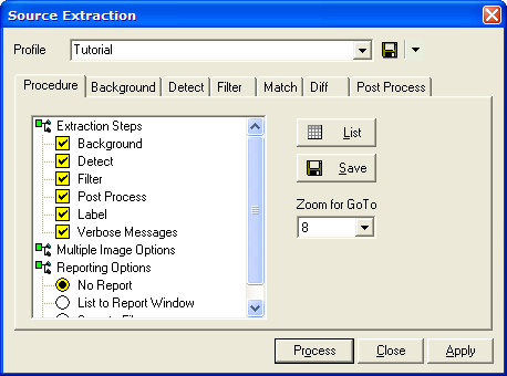
When the profile is loaded, Mira sets all the preferences on on all dialog pages to those values stored in the profile. To see what all dialogs should look like for this tutorial, click here. Note that, in this tutorial, you will not be using the Multiple Images options (Matching and Difference) because only a single image has been loaded. If you double click on Multiple Images to open its options, you will see all options disabled with X marks. As a consequence, the preferences on the Match and Diff pages are not used.
Next, you will run the pipeline using the "Tutorial" profile. With the Source Extraction pipeline dialog open, click [Process]. After some number of seconds, the pipeline finishes and the Source Extraction Messages window opens as shown below:
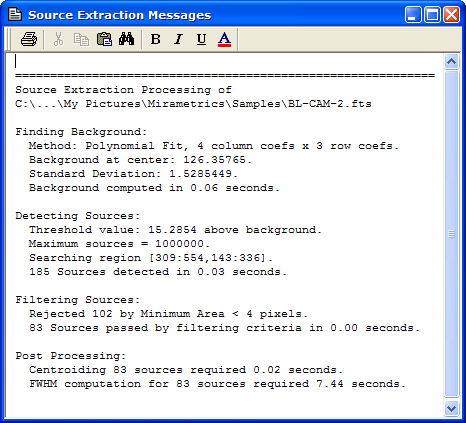
The Messages window was created because the Verbose box was checked on the Procedure page. This is a standard Mira Text Editor window, so the results listed here can be edited or saved for your records.
There are a number of things to be learned from the Messages window. The first interesting point is that 185 sources were identified inside the rectangular region of the image cursor but setting a minimum area of 4 pixels discarded 102 of them, leaving 83 sources 4 pixels or larger. At this low threshold above background, we detected quite a few hot pixels very small object which are mostly just warm pixels You could verify this by re-running the pipeline after unchecking Min Area and setting Max Area = 2 pixels on the Filter page. Second, the Finding, Detecting, and Filtering steps required a very small amount of time to complete, but it took approximately 100 times as long to compute the Precision FWHM values in the Post Processing step. Therefore, if you re-run the pipeline to count the number of tiny bumps, the "computationally expensive" FWHM step is not necessary and should be turned off.
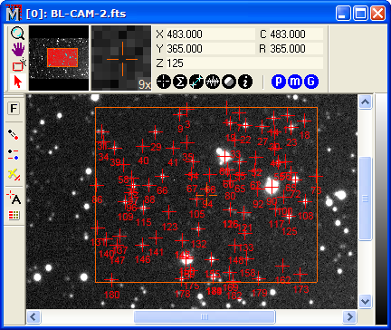
Since the Label step was checked in the procedure, the result of the extraction pipeline looks like the image below, with the final sources marked and tagged with a number. This image was zoomed 2x to give better separation between markers.
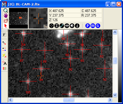
Using the magnify mode or your mouse thumbwheel, zoom the image to 4x so it looks like the picture below. You can now see the kinds of sources that were detected. Notice how bright the faintest objects are compared with the sky noise. This makes it apparent how well Mira's centroiding algorithm works for faint sources. Look at object 68 in particular.
Since we selected Report
Method = "No Report" on the Procedure page, the source properties
extracted from BL-CAM-2.fts were not listed anywhere. Choosing not
to display the results can save time if a large number of objects
are detected, especially if you do not know if you want to save
them (Hint: You can maximize the scrolling speed of the report
window by keeping Auto-optimizing the column widths). However, you
can view the information after the fact. In this case, only 83
sources passed the filtering and that is quick to display in a
Report window. Click ![]() to open the
Source Extraction dialog and select the
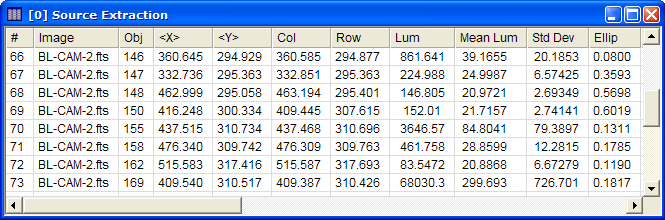
Procedure page. Click the [List] button and the Report window opens as in the picture below
(this is shown scrolled down to object 66). Close the
Preferences dialog so you can continue using the other
windows.
to open the
Source Extraction dialog and select the
Procedure page. Click the [List] button and the Report window opens as in the picture below
(this is shown scrolled down to object 66). Close the
Preferences dialog so you can continue using the other
windows.
If you want to save these results, make sure the Report window is top-most and use the File > Save As command to save it to a text file.
You can do many things with the tabular data in a Report window, including save it to a text file, copying onto the Windows Clipboard, or rearranging the columns and sorting the rows to make comparisons (see Working with Report Windows). In addition, you can create a Scatter Plot to examine relationships between the source properties.
Make the Source Extraction Report the top-most window and click the View > Scatter Plot command in the pull-down menu. You can also access commands like Scatter Plot by right-clicking inside the Report window to open its Context Menu. The Scatter Plot command opens a setup dialog like this one:
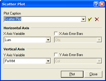
In the Scatter Plot dialog, you select which columns of report data to plot on the horizontal and vertical axes. Optionally, you can also set a title and select columns containing data to be used as error bars. As shown above, use the two left-hand listboxes to select "Lum" as the X Axis Variable and "FWHM" as the Y Axis Variable. This will produce a graph showing FWHM versus Luminance for all the sources that were extracted from the BL-CAM-2.fts image. Click [Plot] to create the graph like this:
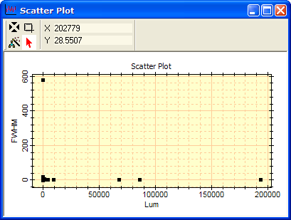
Notice that a single point with FWHM near 600 has
set the plot scale so that the other points are all crunched
together near the bottom. We will investigate this particular
source later. At the moment, let's have a closer look at the other
FWHM values. On the Plot Toolbar, Click
![]() to enter Expand
Mode and drag a rubberband around the plot region to zoom in
as shown below:
to enter Expand
Mode and drag a rubberband around the plot region to zoom in
as shown below:
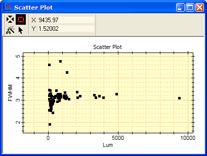
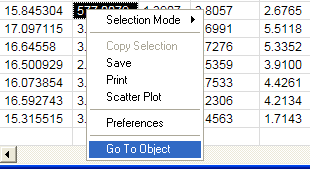
We can see that the typical FWHM is around 3.2 pixels. The increased scatter in FWHM at very low luminance is to be expected because the measurement becomes dominated by sky noise. The higher values of FWHM could be faint galaxies or could just be random fluctuations for very faint stars. We can examine them more closely using the same method we will use for the object we noted above as having a FWHM near 600. Which object is that? You could scroll through the table to find it but there is an easier way. In the Report window, click the FWHM column header to sort the source list by value. If it sorts in the wrong sense, with the smallest value at the top of the list, click again to get the largest value at the top of the list. Right-click on the cell containing the value FWHM value of 577 to open the Context Menu for this Report window. Notice that the value highlights underneath the menu as shown below. In the menu, select Go To Object as shown here:
The Go To Object command shifts the displayed image to the position of the object who's table cell was highlighted. If you expose the Image Window containing BL-CAM-2.fts, you will see it centered as shown below. The zoom value was set on the Procedure page of the Source Extraction dialog.
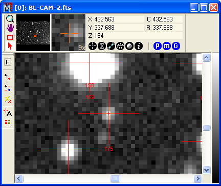
Why did Mira calculate a FWHM value of 577 for this
object? To answer that question, click the ![]() button on the left end of the Image Toolbar to enter
Roam Mode (so that clicking on the image does not execute any
command from a toolbar). Now hold down the Shift key and click the
mouse pointer on the star to center the Image
Cursor at that point. Then click the
button on the left end of the Image Toolbar to enter
Roam Mode (so that clicking on the image does not execute any
command from a toolbar). Now hold down the Shift key and click the
mouse pointer on the star to center the Image
Cursor at that point. Then click the ![]() button on the main toolbar to create
a Radial Profile Plot like the one shown
below.
button on the main toolbar to create
a Radial Profile Plot like the one shown
below.
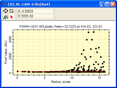
The object of interest is on the left, centered at a radius value of 0. The huge scatter of points on the right correspond to the extremely bright star just above the target star in the Image Window. Notice the FWHM value of 1037 pixels listed in the caption above the plot box. It is clear that the FWHM measurement could not cope with the extremely bright star in the nearby background, which made the measurement invalid.
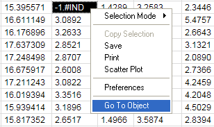
There is another object of interest in this report window. If you sort the FWHM list again, the object at the small end has the value -1.#IND, which is computer speak for a numerical value that could not be computed. Usually this means that the object is just too faint to get a numerically stable solution for the FWHM. Right-click on this value and repeat the Go To Object command.
The Go To Object command centers the Image Window on the point like this:
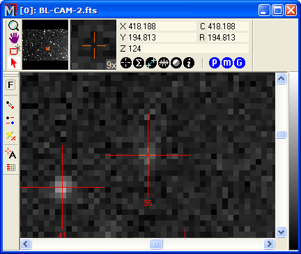
That is one really faint object. Again, the FWHM value could not be calculated because the object was just so faint that the solution gave a nonsensical result. Still, the centroid coordinate appears to be accurate even at this incredibly low brightness level.
In this Tutorial we have shown how to setup and use the MExtract module to detect and extract information about sources in the image. Using a similar strategy but with different parameters such as filtering limits, one can use the Extract Sources command and other Mira tools to do such varied projects as counting bad pixels, characterizing optical aberrations across the field of view, or hunting for galaxies using their higher ellipticity and lower values of CI or higher FWHM as classification criteria.
Getting Started, Extract Sources command, Extracting Sources from Images, Running the Source Extraction Pipeline