Published January 2020
Source Extraction is also known by the names "image segmentation" and "image labeling" in various applications. This procedure identifies, or detects individual objects or image features in one or more images and computes some 40 properties for each detection. Source Extraction provides numerous options for controlling the detection and processing of information. The procedure may also be used to detect objects or features that are common to an image set or that vary among the images. Source extraction is handled using the Source Extraction package in Mira Pro x64.
This tutorial, from the Mira Pro x64 User's Guide, shows how use the Source Extraction package to detect and measure the properties of sources in images. The Source Extraction package is accessed using the Measure > Extract Sources command for an Image Window. The Source Extraction Package is immensely powerful and has a great number of important and varied applications. In this tutorial it is used simply to examine the FWHM values for many stars in a small region of an astronomical image. A quick overview of the extraction procedure is described in the User's Guide topic, "Running the Source Extraction Pipeline."
Overview
Source extraction involves the detection and measurement of all sources brighter than a threshold value. This processing uses a chain of operations called a "pipeline". Each step in the pipeline involves Properties that control its operation. Because Mira allows so many variations for the steps used in the pipeline, a Profile control is used to manage the procedure. The pipeline is operated from the Source Extraction Properties. After you have choose a profile or set your Properties, you run the pipeline by clicking the [Process] button.
The source extraction pipeline creates a procedure for each selected processing step. The steps you select are applied in a specific order, hence the term "pipeline" to describe a single direction of flow in the processing. The first step in source extraction involves determining the background level. Knowing the background at each point, each pixel can be tested against the threshold above background; if the pixel exceeds the threshold, it is tagged as a source candidate. All candidate pixels are then collected into sources completely separated from others by a boundary at the specified threshold level. In this way, the sources are like islands poking above sea level. Source properties such as intensity, ellipticity, area, and others are then computed. The final processing step involves filtering this source list to retain only the sources that meet criteria such as being within a certain range of area or ellipticity. The list of sources extracted from the image(s) may then be further analyzed using Mira tools or saved for analysis by other software.
Getting Started
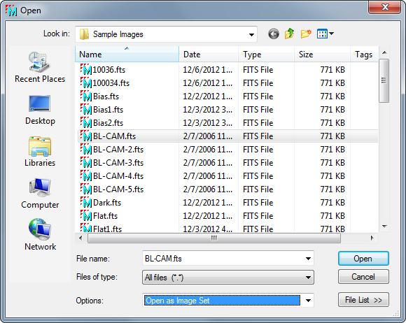
To begin, use the File > Open command to load the Open dialog. As shown below, select the sample image BL-CAM.fts. Before opening the image, be sure the "Flip FITS Image" option is not checked in the Options list at the bottom of the Open dialog. Then click [Open] to display the image in Mira.
After opening the image, click
![]() on the main toolbar or use the Measure > Extract Sources command
in the menu. This opens the Source Extraction Toolbar which operates all
the commands of the
Source Extraction package. As typical in Mira, the toolbar opens on the
left border of the image window with marking mode active:
on the main toolbar or use the Measure > Extract Sources command
in the menu. This opens the Source Extraction Toolbar which operates all
the commands of the
Source Extraction package. As typical in Mira, the toolbar opens on the
left border of the image window with marking mode active:
Use the Image Cursor Properties dialog to adjust the Image Cursor as shown above, to a size of 250 x 200 pixels and centered at coordinate (431,241).
The toolbar commands are described below. In this tutorial, the only buttons you will use are the first and last ones:
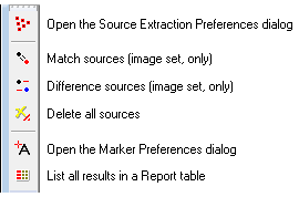
Notice that this toolbar has no "marking mode", as is usually the top-most button on the toolbar. Source extraction does not involve an interactive marking mode. However, the top-most button does open the Source Extraction Properties which you use to automatically identify and extract the source information.
Loading the Tutorial Properties
Next, we will load the extraction Properties to be used in this
tutorial. On the toolbar, click the
![]() button to open the Source Extraction dialog. Now you need
to set the values on all the pages of the dialog. The Profile control makes this
easy. The tutorial Properties have been pre-defined and stored in the profile
named "Tutorial". At the top of the dialog, click the drop arrow and select
"Tutorial" as shown below. Be certain the
Use Cursor ROI
box is checked so that only the cursor is searched for sources.
button to open the Source Extraction dialog. Now you need
to set the values on all the pages of the dialog. The Profile control makes this
easy. The tutorial Properties have been pre-defined and stored in the profile
named "Tutorial". At the top of the dialog, click the drop arrow and select
"Tutorial" as shown below. Be certain the
Use Cursor ROI
box is checked so that only the cursor is searched for sources.
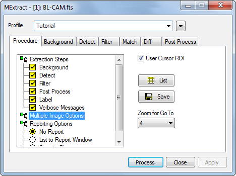
When the profile is loaded, Mira sets all the Properties on on all dialog pages to those values stored in the profile. In this tutorial, you will not be using the Multiple Images options (Matching and Difference) because only a single image has been loaded. If you double click on Multiple Images to open its options, you will see all options disabled with X marks. As a consequence, the Properties on the Match and Diff pages are not used.
Running the Extraction Pipeline
Next, you will run the pipeline using the "Tutorial" profile. With the Source Extraction pipeline dialog open, click [Process]. After a moment, the pipeline finishes and the Source Extraction Messages window opens as shown below:
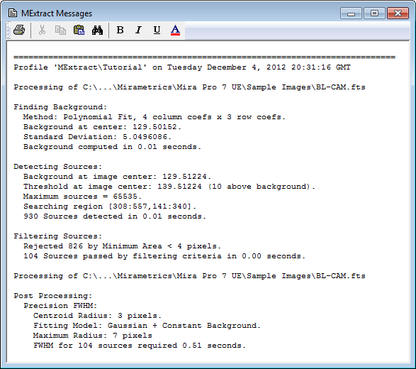
The Messages window was created because the Verbose box was checked on the Procedure page. This is a standard Mira Text Editor window, so the results listed here can be edited or saved for your records.
There are a number of things to be learned from the Messages window. The first interesting point is that 930 sources were identified inside the rectangular region of the image cursor but setting a minimum area of 4 pixels discarded 826 of them, leaving 104 sources 4 pixels or larger. At this very low threshold above background, a large number of hot pixels were detected. You could verify this by re-running the pipeline after unchecking Min Area and setting Max Area = 2 pixels on the Filter page. Second, the Finding, Detecting, and Filtering steps required negligible time to complete, but 0.51 seconds was required to compute the Precision FWHM in the post-processing step. If you re-run the pipeline to count the number of tiny bumps, the "computationally expensive" FWHM step is not necessary and should be turned off.
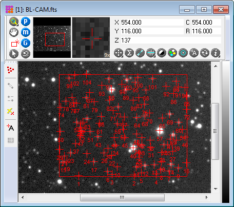
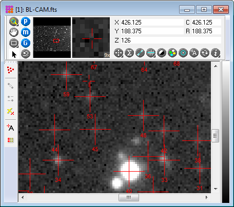
Since the Label step was checked in the procedure, the result of the extraction pipeline looks like the image below, with the final sources marked and tagged with a number. This image was zoomed 2x to give better separation between markers.
Using the magnify mode or your mouse thumb wheel, zoom the image to 4X so it looks like the picture below. You can now see the kinds of sources that were detected. Notice how bright the faintest sources are compared with the sky noise. This makes it apparent how well Mira's centroiding algorithm works for faint sources. For example, see sources 44 and 45 in the image below.
Since we selected Report Method =
"No Report" on the
Procedure page, the source properties extracted from
BL-CAM-2.fts were not listed anywhere. Choosing not
to display the results can save time if a large number of sources are detected,
especially if you do not know if you want to save the results (Hint: You can
maximize the scrolling speed of the report window by keeping Auto-optimizing the
column widths). However, you can view the information after the fact. In this
case, only 83 sources passed the filtering and that is quick to display in a
Report window. Click
![]() to open the
Source Extraction Properties
and select the
Procedure page. Click the [List] button and the
Report window opens as in the picture below (this is shown
scrolled down to source 66). Close the Properties
dialog so you can continue using the other windows.
to open the
Source Extraction Properties
and select the
Procedure page. Click the [List] button and the
Report window opens as in the picture below (this is shown
scrolled down to source 66). Close the Properties
dialog so you can continue using the other windows.

If you want to save the se results, make sure the Report window is top-most and use the File > Save As command.
Analyzing the Extraction Data
You can do many things with the tabular data in a Report window, including saving it to a text file, copying onto the Windows Clipboard, or rearranging the columns and sorting the rows to make comparisons (see Grid Controls). In addition, you can create a Create Plot from Grid to examine relationships between the source properties.
Make the Source Extraction Report the top-most window and click the View > Create Plot from Grid command in the menu. The Create Plot from Grid command opens a setup dialog like this:
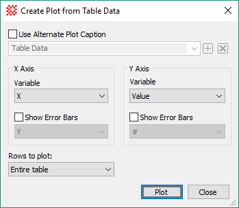
In the Create Plot from Grid dialog, you select which columns of report data to plot on the horizontal and vertical axes. Optionally, you can also set a title and select columns containing data to be used as error bars. It would be interesting to examine whether the FWHM value depends on the Ellipticity of the star. To do this, use the two left-hand list boxes to select "Ellip" as the X Axis Variable and "FWHM" as the Y Axis Variable. This will produce a graph showing FWHM versus Ellipticity for all the extracted sources. Click [Plot] to create the graph like this:
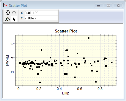
We can see that the typical FWHM is around 3.2 pixels and shows no obvious trend as a function of the Ellipticity.
Previously sources 44 and 45 were mentioned as being quite faint. What is the faintest source detected? To get an answer, select the Source Extraction report window and click the Lum column header to sort the table by Luminosity. This puts Source 29 at the top of the list as being the faintest source. To locate this source in the image, right-click the table row of the Source 29 to open the window's context menu. Select Go to Object as shown here:
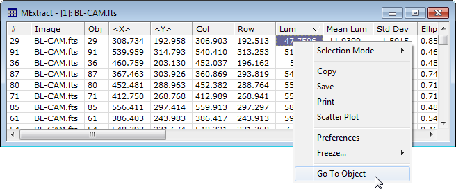
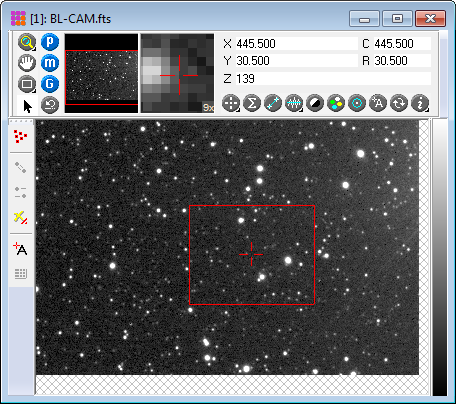
The Go To Object command shifts the displayed image to the coordinates of the source who's table row was clicked (note: this is different from the Go to Object command in the Coordinates menu). If you expose the Image Window containing the BL-CAM.fts image, you will see it centered as shown below. The magnification value was set on the Procedure page of the Source Extraction Properties.

What is the FWHM value for this source? Hold down the Shift key and click the mouse pointer on source 29 in the Image Window. This moves the Image Cursor to Source 29. Right click on the image to open the Image Context menu and select the Plot > Radial Profile command to create a Radial Profile Plot like the one shown below.

The FWHM of 3.958 for the incredibly faint Source 29 is slightly larger than the average for the sources detected.
In this Tutorial you have learned how to setup and use the Source Extraction Package to detect and extract information about sources in an image. Using a similar strategy but with different Properties such as filtering limits, one can use the Measure > Extract Sources command and other Mira tools to do such varied projects as counting bad pixels, characterizing optical aberrations across the field of view, or hunting for galaxies using their higher ellipticity and lower values of CI or their higher FWHM as classification criteria.