Tutorial: Creating Plots from Images
This tutorial teaches you how to create luminance plots from images. In this exercise we will make Line Profile plots and Row Profile plots from one of the sample images. For further information about plotting, see Plotting Commands, Working with Plots, Plotting Examples, and Examples of Row Plots.
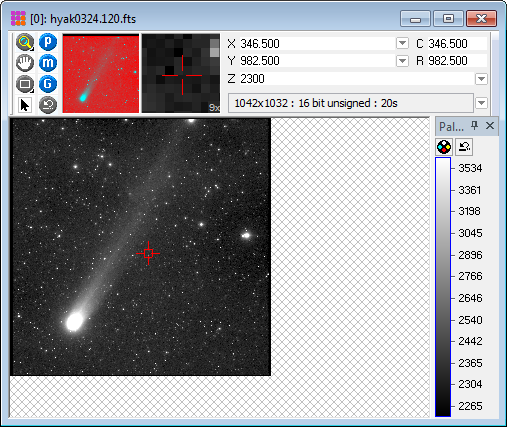
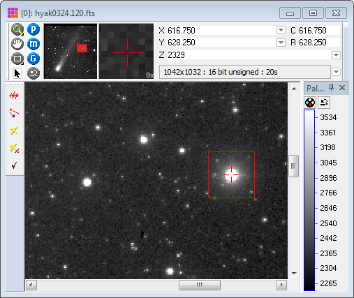
To create a plot, we need to first display an image (see Tutorial: Displaying an Image). After starting Mira , click the File > Open command in the main menu bar. This opens the normal the Open dialog. In this dialog, navigate to the sample images in the folder "<Documents>\Mira AL\Sample Data". Open the image named'hyak0324.120.fts'. The displayed image will look like the one shown below. Note that the image may appear larger or smaller than shown here, depending upon how Mira scales it to fit the screen.
Open the Line Profile Toolbar for this Image Window using the either menu command or button on the Image Plot Toolbar. Now magnify and re-center the image so that it appears as shown below:
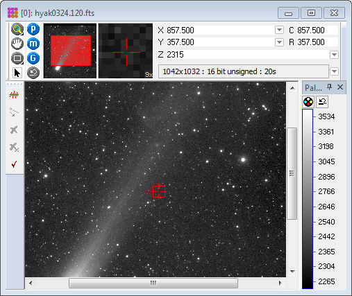
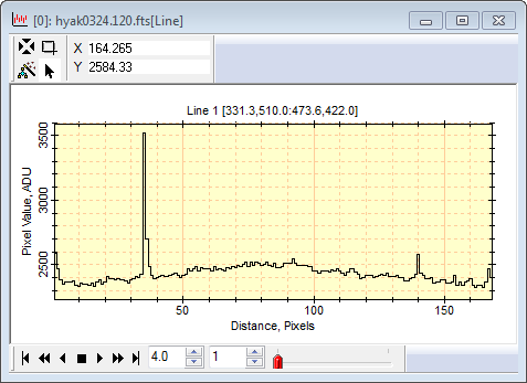
A Line Profile Plot shows the change in luminance along a line drawn on the image. This type of plot uses the Line Profile Toolbar shown on the left side of the Image Window in the figure above. This is a standard Command Toolbar which was opened by clicking on the Image Plot Toolbar at the top of the Mira application window. This toolbar opened in the typical mode with the top button (the marking mode) enabled. Using these toolbar buttons you can plot the luminance along any vector drawn on the plot and, as with other Mira plots, it works for both RGB images and non RGB images. To make a plot, mouse simply down at the starting point, then drag the line to its ending point and release the mouse. You will get a plot that looks like this:
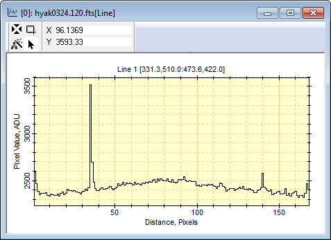
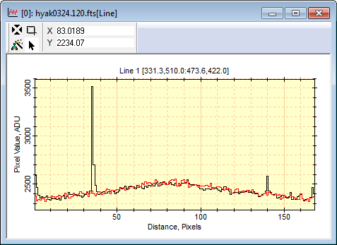
Next we want to know what is happening to pixels along a parallel line beside the line we just drew on the image. Click the second button on the toolbar to enter Move Mode. Next, point the image cursor at the line then click and hold down the mouse button, to grab the line marker on the image, and drag the line to a new location. When the mouse is released, the new profile is added to the existing Plot Window. If you see only the same plot after doing this, right click on the plot and selectPlot Series Mode > Overplot. The plot should then look as follows:
We can continue adding plot series and watch each
one add to the plot window. The Image Window is in the toolbar
mode, meaning that each time you click on the image the current
toolbar command mode (move and draw a new line) will be executed.
To get out of that cycle so you can freely click on the image,
click ![]() on the Image Window to return to
deactivate all modes. If you don't like the scaling, labels, or
appearance of the Plot Window, press Ctrl+A to open the Plot Properties dialog. If you do not like the
colors or thickness of the lines, pressCtrl+Shift+A to open the Plot Series
Properties dialog.
on the Image Window to return to
deactivate all modes. If you don't like the scaling, labels, or
appearance of the Plot Window, press Ctrl+A to open the Plot Properties dialog. If you do not like the
colors or thickness of the lines, pressCtrl+Shift+A to open the Plot Series
Properties dialog.
When more than 1 plot series exists, you can choose to Animate them or Overplot them. Right click on the plot to open the Plot Context Menu and select Plot Series Mode > Animate or Plot Series Mode > Overplot This command changes the window between these two forms:
When the Animate mode is active, notice the Animation Pane at the bottom of the Plot Windows. Using Overplot and Animate modes in is a conceptually similar to working with an Image Set in an Image Window. Essentially, the Plot Series act like an Image Set.
Next, let us plot the profile of a single row
through the peak of a star. To make a Column Profile Plot or Row
Profile Plot, we use the Image Cursor to mark the extent of the
plot. To plot a Row Profile, you must first adjust the Image Cursor
to enclose the columns and rows you want to use. Often we would do
that by moving and sizing the Image Cursor. In this case we may
want to set the length of the plot (the number of columns) and we
want to position it on the peak of a star. In the Image Window, switch to
Cursor Mode and move
the cursor onto the star as shown below. Then click ![]() on the Measurements Toolbar
to center the cursor on the star as shown below.
on the Measurements Toolbar
to center the cursor on the star as shown below.
In terms of centering the Image Cursor on a peak (or valley) such as a star, there are several ways to do this:
One way is to have a steady hand and carefully position the image cursor using by microscopic mouse movements while watch for the peak pixel value to appear in the Image Toolbar.
Another method is to magnify the image so it is easier to position the mouse on the center of the star. You can use the mouse to position the Image Cursor or, if the window has focus, you can position it using the keyboard arrow keys. The window does have focus if you have clicked on it.
Still another method is to crudely position the
Image Cursor within a few image pixels of the peak. Then click
![]() on the Measurements Toolbar
to home theImage
Cursor to the centroid position near where you dropped it with
the mouse.
on the Measurements Toolbar
to home theImage
Cursor to the centroid position near where you dropped it with
the mouse.
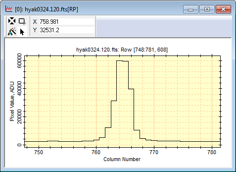
Now that the Image cursor is positioned on a star,
click ![]() on the Image Plot Toolbar to
plot the single row at the center of the Image Cursor. This button
executes the Row Profile Plot command. Clearly Method 3, above, is
the quickest way to get a row profile plot through the center of a
star. And it shows why some commands such as Centroid , Statistics,
and Profile Plots are all linked to the Image Cursor. Notice that
the plot caption (not the window caption) reminds us of the columns
and rows we just plotted. In this case, [748:781, 608] tells
us that we plotted from column 748 through 781 along row 608. Since
we centroided before making the plot, the center of the plot passes
through the peak of the star profile.
on the Image Plot Toolbar to
plot the single row at the center of the Image Cursor. This button
executes the Row Profile Plot command. Clearly Method 3, above, is
the quickest way to get a row profile plot through the center of a
star. And it shows why some commands such as Centroid , Statistics,
and Profile Plots are all linked to the Image Cursor. Notice that
the plot caption (not the window caption) reminds us of the columns
and rows we just plotted. In this case, [748:781, 608] tells
us that we plotted from column 748 through 781 along row 608. Since
we centroided before making the plot, the center of the plot passes
through the peak of the star profile.
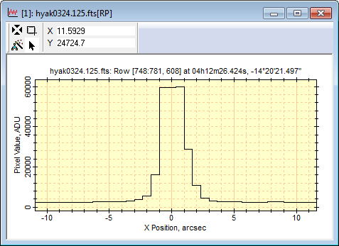
The plot above would have different axes if the
image had a world coordinate calibration and the plot was created
using World Coordinates. Provided that the image has a World Coordinate
System calibration, with Right Ascension and Declination for
every point, then you can choose to plot in those coordinates. The
choice is specified a number of places in Mira , one being in the
Image Context Menu > Plot menu. Right click on the image
to open the Image Context Menu, select the Plot submenu,
then the check the World Coordinate
item. Then click ![]() again, and a plot
is created like the one below with World Coordinate position on the
X axis. Roaming the mouse pointer around either plot lists the
coordinates in whichever Plot Coordinate System was used.
again, and a plot
is created like the one below with World Coordinate position on the
X axis. Roaming the mouse pointer around either plot lists the
coordinates in whichever Plot Coordinate System was used.
To plot using world coordinates (assuming the image is calibrated in world coordinates), the plot mode must be set to World Coordinates mode. To do this, open the menu for the plot command you want to use, then select Coordinate Mode > World. Then make the plot. The To make the plot below, a sample image having a world coordinate calibration was opened. The following example shows a world coordinate plot made from the same star but in a different sample image having a world coordinate calibration,hyak0324.125.fts .

The tutorial Displaying an Image Set shows how to overplot the row profiles for members of an image set.
The previous sections have described how to Overplot multiple line profiles by using Move mode for the Line Profile Plot. This technique is useful for comparing different plots directly from different points in an image, different images, or for comparing different types of plots.
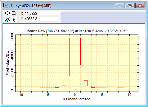
The following example shows how to switch the plot averaging mode to create and compare a single row plot with a median row plot across the same star profile. The image used has a world coordinate calibration so the plots were created using it. First, create a plot of a single row through the center of a star as in the previous examples:
Now click the black arrow next to the Row Profile Plot button on the Image Plot Toolbar to open the drop menu. If the menu shows a command for Median Row then click on it. If some other method is shown (see Mean Row in the picture below), then you need to change it. To make the change, select Averaging Mode > Median as shown below, then re-open the menu and click the Median Row command .
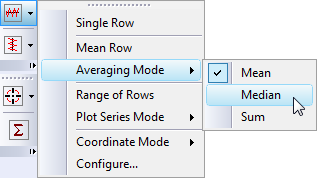
After changing the Averaging Mode, the menu re-opens showingMedian Row in place of Mean Row as shown above, before making the change. Click on Median Row to create the median row plot:
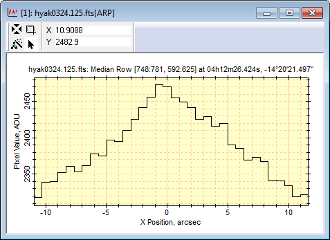
In the two plots above, compare the Y axis scales to see the difference in range between a single row and the median over all rows. Obviously, the median rejects the high pixel values as being outliers, so it has a smaller range.
Next, we will use the Copy + Paste method to combine the two plots in the same plot window for direct comparison. Here is the procedure:
Click the window containing the mean row plot to make it top-most and use the menu command Edit > Copy (Ctrl+C) to copy the mean plot data to the Windows clipboard.
Click on the window containing the median row plot to make it top-most and useEdit > Paste (Ctrl+V) to paste the mean row plot as a new series in the median row plot window.
The result looks like the following:
The window above shows both row plots overlaid on the same set of axes; this is called "Overplot Mode".
Mira offers two plotting modes, Overplot and Animate, which you can select using thePlot Series Mode command in the right-click Plot Context Menu. The colors and other attributes of the plot series can be changed using the Plot Series Properties command in the same menu. See Plot Windows for details about these and other features.
Contents, Tutorials, Getting Started, Tutorial: Displaying an Image Set, Plotting Commands, Examples of Row Plots