Michael Newberry
Copyright © 2008. Mirametrics, Inc., All Rights Reserved.
The overscan bias correction provides a highly accurate way to correct the bias signature of a CCD image. The value of using the overscan method is that it corrects the bias in each row of the image at the time it was read from the CCD camera. To estimate the electronic bias of the CCD, it may be "overscanned" by adding dummy reads of the electronics without the presence of physical pixels. Repeating the dummy reads for the entire chip adds 1 or more lines of data which might be generally called overscan lines. Overscanning the horizontal register adds columns to the image that may be used to perform a column bias correction. Reading dummy rows before or after the physical CCD can be used to perform a row bias correction. Since the CCD can be considered a horizontal state machine, significant bias structure usually appears along columns, as a function of row number. For this reason, the column bias method is most widely used and it is described below.
Overview
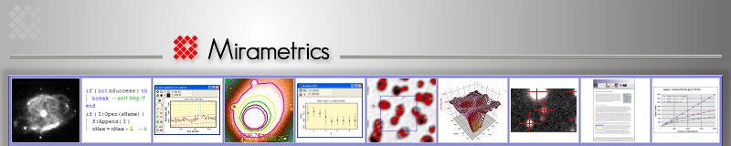
The picture below shows a sample image kindly provided by Jim Moronski of Finger Lakes Instrumentation. This image was a flat field frame taken with an engineering grade CCD but it serves to show how to perform an overscan bias correction. The black region to the right of the main image is the overscan region. It has a significantly lower signal level because it contains only bias whereas the main image contains bias plus dark current and light.
 In
the picture at left, the red rectangle shows the columns that will be used in the analysis below. The
rectangle is 100 columns wide and runs almost the full height of the
CCD. Since the overscan region extends over 400 columns, a wider
rectangle could have been used. However, 100 columns was adequate
for the purpose.
In
the picture at left, the red rectangle shows the columns that will be used in the analysis below. The
rectangle is 100 columns wide and runs almost the full height of the
CCD. Since the overscan region extends over 400 columns, a wider
rectangle could have been used. However, 100 columns was adequate
for the purpose.
Procedure and Strategy
Performing a column bias correction involves 3 main steps:
- Determine the columns to use in sampling the overscan.
- Determine parameters of a polynomial function that adequately characterize the bias as a function of row number.
- Compute and subtract the polynomial function from every pixel of the CCD image.
Steps 1 and 2 need be done only once for a given camera and image size. Since the overscan correction maps the bias applied to each specific row of each image, it needs to be corrected individually for each image. However, the general shape of the overscan bias varies only slightly between images acquired using the same camera setup. Therefore, the strategy for correcting bias is to determine the parameters of a good fit (steps 1 and 2) and then blindly compute and apply the fit specifically for each individual image (step 3). It needs to be emphasized noted that a formal analysis as described in steps 1 and 2 needs to be done at least once for a given camera, binning, and subframe setup before the blind correction described in step 3 can be trusted.
Why correct the bias using a smooth polynomial function of row number? Why not just measure the average bias value in each row and subtract that value from the entire row? The answer to these questions is that each pixel contains noise, so the bias value estimated for a row shows statistical fluctuations. If you subtract it directly from the entire row, you will add streaks to the image that should not be there. Assuming that the bias really is a slowly varying function of row number and does not take wild jumps from one row to the next, the polynomial uses information from neighboring rows to obtain a far more significant estimate of the bias in each row.
Determining the Column Sampling Region in the Overscan
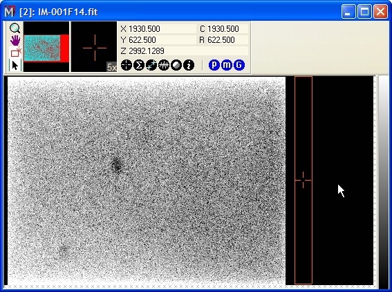
To perform step 1, we need to determine where to place the overscan sampling rectangle. When
clocking out the CCD, there is a tiny residual charge that is not
transferred from one pixel to the next during serial readout. This
accrues across the width of the CCD and gets dumped into the first
columns of the overscan. It shows an exponential tail that decays
down to what is essentially the overscan bias level by some
particular column number. Which column is this? We
 determine this by
making an average row plot of pixels inside the rectangle (this
means that each point in the plot consists of the average of all
rows at that column number). The picture at left shows this average row
plot. It appears that the overscan decays to an essentially constant
bias value by around column 1680. In the picture of the image above,
the rectangle has been positioned to start at column 1680. We use a
rectangle of 100 columns so that values we measure in the bias are
averaged over many columns to increase their statistical significance
(in other words, to beat down the random errors).
determine this by
making an average row plot of pixels inside the rectangle (this
means that each point in the plot consists of the average of all
rows at that column number). The picture at left shows this average row
plot. It appears that the overscan decays to an essentially constant
bias value by around column 1680. In the picture of the image above,
the rectangle has been positioned to start at column 1680. We use a
rectangle of 100 columns so that values we measure in the bias are
averaged over many columns to increase their statistical significance
(in other words, to beat down the random errors).
A First Look at the Overscan Bias
The graph below shows a column plot along a single column at the
center of the red rectangle. The black values show the pixel values
and they appear to follow a slope plus some curvature. The red curve
shows a 3 term polynomial fit (the quadratic y = a0 + a1x
+ a2x2). All points were fit (none rejected),
giving a standard deviation of the fit is +/- 25.4 ADU, which is
then an excellent estimate of the readout noise. Data rejection is
not usually warranted because the bias is a
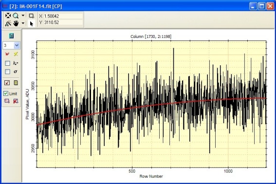 smooth function of row
number plus or minus readout noise.
smooth function of row
number plus or minus readout noise.
Is this fit adequate to characterize the bias or is there finer structure that is hidden by the noise in a single column? By averaging many overscan columns to beat down the noise, we will be able to reveal lower level structure.
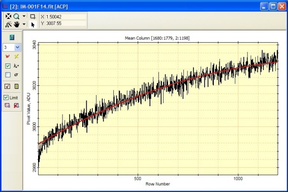 The next plot shows the mean column value in the overscan rectangle
plus a fit. Notice that the reduction in noise reveals finer
structure as expected. As above, the red curve shows a 3-term
polynomial fit with a standard deviation of 2.64. Notice that the
highest and lowest rows do not show the brightening visible in
original image, revealing that edge effect results from dark current, not bias.
The next plot shows the mean column value in the overscan rectangle
plus a fit. Notice that the reduction in noise reveals finer
structure as expected. As above, the red curve shows a 3-term
polynomial fit with a standard deviation of 2.64. Notice that the
highest and lowest rows do not show the brightening visible in
original image, revealing that edge effect results from dark current, not bias.
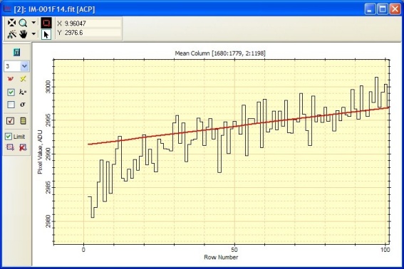 The plot at left shows an enlargement of the lower left portion of the
plot above. This shows the bias turning downward, away from the fit
below row 30.
The plot at left shows an enlargement of the lower left portion of the
plot above. This shows the bias turning downward, away from the fit
below row 30.
Improving the Overscan Bias Correction
To get a more accurate mapping of the bias correction, the number of polynomial terms must be increased. The plot at left
shows the same data with
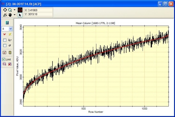 an 8 term polynomial fit. The fit order was increased until the turndown below row 30 was acceptably handled.
The improved fit has a standard deviation of
2.51. The small reduction in standard deviation results primarily
from obtaining a better fit below row 30.
an 8 term polynomial fit. The fit order was increased until the turndown below row 30 was acceptably handled.
The improved fit has a standard deviation of
2.51. The small reduction in standard deviation results primarily
from obtaining a better fit below row 30.
Applying the Overscan Bias Correction
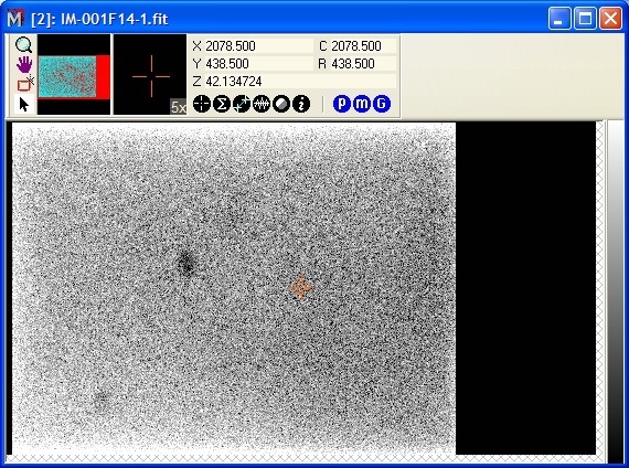 The picture at left shows the 8th order fit to
row number subtracted form every column of the image. In this view, you can't discern
much difference between the corrected image and original image as bias variations are
dominated by far greater dark current. However, detailed scientific measurements are compromised
unless the additive bias signature is not correctly isolated from the
multiplicative effects of dark current and scattered light. As a final
cosmetic correction, the bias overscan region can be trimmed away as
it is no longer needed and just adds size to the image file.
The picture at left shows the 8th order fit to
row number subtracted form every column of the image. In this view, you can't discern
much difference between the corrected image and original image as bias variations are
dominated by far greater dark current. However, detailed scientific measurements are compromised
unless the additive bias signature is not correctly isolated from the
multiplicative effects of dark current and scattered light. As a final
cosmetic correction, the bias overscan region can be trimmed away as
it is no longer needed and just adds size to the image file.
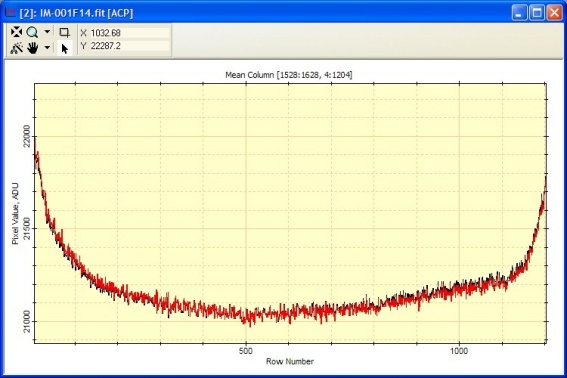 The graph
at left shows a column section of the bias corrected image
and the original image. The black curve shows the original image and
the red curve shows the bias corrected image. The difference between
these curves equals the polynomial fit that was computed from the overscan in the original image.
The graph
at left shows a column section of the bias corrected image
and the original image. The black curve shows the original image and
the red curve shows the bias corrected image. The difference between
these curves equals the polynomial fit that was computed from the overscan in the original image.